Wednesday, April 27, 2016

Primary Vote Tallies: 4/27/2016

Last night the results came in from the Northeast version of the "Super Tuesday" primary for both parties, GOP & Dem: CT, DE, MD, PA & RI. Trump swept all states with percents in the 50s & 60s, while Clinton took four states. On one hand, it has been claimed that turnout is greater than in other recent primaries, indicating a surge in political interest this year, but on the other hand, 538 claims that turnout in the primary is unrelated to turnout in the general election. From the candidate's perspective, Trump has claimed that he has "millions more" votes than Cruz.

There are numerous ways to look at each of these claims. In general, each of the claims is true, and as of the most recent votes (4/26/16), they remain true. However, digging into the data can produce interesting results--I have provided two data table below of all of the state votes so far: the first are sum totals by candidate, and the second is all of the data at the state level. Total, Clinton has received the most votes of any individual candidate, and she can make Trump's claim, that she has "millions more" votes than Trump. She also has "millions more" votes than Cruz and Kasich combined. Sanders has more votes than Cruz or Kasich separately, but fewer votes than Trump. Clinton and Sanders combined have received more votes than Trump, Cruz and Kasich combined.

Clinton12,173,896
Trump9,972,683
Sanders8,980,077
Cruz6,777,746
Kasich3,641,272
Cruz+Kasich10,419,018
Clinton+ Sanders21,153,973
Trump+Cruz+Kasich20,391,701

Then table below is the data I used for this analysis. There are some important caveats in the totals I presented above. First, there are states where raw citizen vote numbers for one or both parties simply aren't published. For example, Alaska, Wyoming and Colorado provide only delegate convention votes for either the Dem or GOP side, or both. I have excluded those states from the table. Second, some states have only had a primary/caucus for one of the parties, such as Kentucky, Nebraska and Washington. I have excluded those states from the count as well. Third, I have intentionally excluded counts for any other delegates, like O'Malley on the Democrat size, or Rubio, Carson, etc, on the Republican side. I make no claims for the total GOP or Dem totals if you factored in those votes, or the votes from the states I excluded.

StateBernie SandersHillary ClintonDonald TrumpTed CruzJohn Kasich
Alabama7639930992837173518060837970
Arizona16340023569724991613214753040
Arkansas6486814458013314412387315098
Connecticut36659559501225192477960447
Delaware152895169763424721111014225
Florida56660310974001077221403640159412
Georgia21433254300850170730510972303
Hawaii2353010125680550631566
Idaho1864050656247810094216517
Illinois9820171017006556916434038282874
Iowa852558574545427516663474
Kansas264501259317062352077795
Louisiana7224022161512481811394919355
Maine22311232607085502270
Maryland28127553324723662382038100089
Massachussets58671660378431131360473113783
Michigan595222576795483751330015321655
Minnesota1181357351024018326846488
Mississippi3634818244719175514706535817
Missouri30907131060238209338036792533
Nevada5678631634531160792709
New Hampshire151584952521004063318944909
New York7634691054083524932126151217904
North Carolina460316616383458151418740144299
Ohio513549679266727585267592956762
Oklahoma17405413933813014115794116515
Pennsylvania719911918649892702340201304793
Rhode Island667205249339059639314929
South Carolina9597727151423985116479056206
Tennessee12033324530433270221115945243
Texas4755619350807576181239370120257
Utah61333156662486412256729773
Vermont1158631833519968592918543
Virginia27550750335835596017319396519
Wisconsin567936432767386370531129155200

Saturday, April 9, 2016

Regressing Kasich

I have been posting regression models that fit/predict the presidential primary races by state. Most recently, on the GOP side, four models that use between 3-5 variables each, correctly fit almost all of the states that had voted as of last week, and on the Democratic side, four models that use between 4-5 variables each, also correctly fit almost all of the states that had voted up to, but not including Wisconsin (all of which correctly predicted Sanders' win there). I have so far ignored Kasich, since it was clear early on that he would not gain enough state-level votes to get the presidential nomination on the first ballot. However, since the algorithm I developed makes it easy to plug in the other candidates, I decided to put Kasich through the models.

There is an important difference between all of the other models on both sides that I have produced so far, and the predictions to the right for Kasich. In prior models, I have used the dependent variable of the leading candidate minus the second candidate--thus, Clinton-Sanders, and Trump-Cruz. The resulting fits/predictions are of the difference between those two candidates, not a fit/prediction of the actual percent of win for the candidate. For Kasich, I have created the models based solely on his percent wins for each state. Using the same base of 3,000 variables, and preferencing models that have good statistical values, such as low residuals and BIC, and high adjusted r-squared, as well as a diversity of the "type" of variable used (jobs vs demographics, etc), to the right you will find the fit/predictions for all 50 states, and below you can find the statistical data about each model. All models have significance of p<.001, and all coefficients have significance of p<.01 (most are p<.001). Similar to the prior models, I used about 3,000 variables as the starting point, and while there were a number of very good models that were produced, I present one 2-variable, one 3-variable, and one 4-variable model. I did not test any higher order models.

There are some interesting, and unlikely predictions in some of the models. For example, Kasich2 & Kasich3 (the second and third models) both predict that Kasich will get 50% in New Jersey--a highly unlikely eventuality. Similarly, both models predict negative teens in North Dakota. Clearly, he cannot get negative votes, however, those models are very pessimistic at his success there. Both models provide fairly similar predictions, despite the fact that there is only one common variable between the two models--the percent of women in wholesale drug and chemical business in those states.

One of the unique features of the Kasich models, compared to both the Clinton-Sanders & the Trump-Cruz models, are that in the best Kasich models, I repeatedly found high ranking variables that described women in the workplace. For the previous models, the dominant jobs variables always described men in the workplace. The only male variable in the Kasich models is the broadest of the jobs measures I used, the change in the number of men's jobs from 2000-2013. The women's variables were specific to the last few years, and not a change in the jobs over time. For men, a decrease in the number of jobs, as shown in Kasich1, indicates that Kasich will do better in that state. In Kasich 2 & 3, more women in specific jobs compared to men, like wholesale drugs and chemicals, tends to signal better performance for Kasich.

There were several demographic variables in the high ranking models. The most common were those that designated a change in population and the percent of White Evangelicals. For population change, the second two models indicate that Kasich does better in states with decreasing populations, either from general population decline, or from out-migration. For religion, specifically the measure of White Evangelicals, Kasich does better in states with fewer of them. Economically, Kasich does better in states with higher costs of living. Interestingly, he does better in states where Black families have lower incomes. No other family income measure had a significant predictive utility for the Kasich models.

Thursday, April 7, 2016

Republican Presidential Primary Models: April

Last week I published new models for the Democratic presidential nomination race--here are the new Republican models, updated to include Wisconsin and a broader set of variables. Like the new Democratic models, I de-emphasized theory-building, and generated models that have the best fit of the states which have voted so far, specifically, by including models that use very specific types of jobs variables, like "men in agriculture, forestry and mining (2009-14)," & "change in the number of men in mining jobs (2000-13)." While one can plausibly build a theoretical case for why jobs data is related to the Republican race, it is far more difficult to explain why these specific jobs built statistically significant regression models, while related jobs variables did not. However, even including these jobs variables into the analysis, the best models were largely similar to the last set of models from March 23.

The first table, to the right, shows the state-level predictions/fits for the four models. The first column is the state, and the 2nd column shows the votes that have taken place so far. This is a simple subtraction of Trump-Cruz. It does not account for other contenders, such as votes that Rubio or Kasich have received. A positive number means that Trump beat Cruz by this margin, while a negative number means that Cruz beat Trump by this margin. The numbers highlighted in pink in the next 4 columns are the states this model incorrectly fits. So, for example, Rep1 got Louisiana and Maine wrong--it predicted that Maine would go for Trump, when it actually went for Cruz. Similarly, Rep4 gets 1 state wrong--also Maine. Rep2 and Rep3 correctly fits all 32 states that have voted so far in the Republican race. At the bottom of the page, the next table, lists the specific variables used in each model, and statistical information about each model.

The first model, Rep1, is the most efficient model--it uses only 3 variables, and only gets 2 states wrong, as mentioned above. It uses the percent of young women in the state, employment, and men in agriculture, forestry and mining. As with the previous models, employment & unemployment are important predictors of the Trump-Cruz race. In the prior models, I used unemployment, and the beta-coefficient was positive--meaning that in states where unemployment was high, Trump tended to beat Cruz, and vice versa. In the new models, I used employment, and as predicted, this coefficient is negative, describing that in states where employment is low, Trump does well, but in states with high employment, Cruz does better. This can be seen in specific jobs numbers found in each model. In Rep1, as the number of men in agriculture, forestry and mining (AFM) jobs goes down, Trump does better. In Rep2, as the number of men in mining jobs declines, Trump does better. Not all jobs had this pattern, or showed this level of statistical significance. The effects for women's employment was also not nearly as statistically significant in the Republican race, compared to the effects of men's employment. In Rep 1, the beta-coefficient shows that the AFM jobs variables is the strongest predictor, while the general employment variable is about half that. A test of the VIF (variance inflation factor) showed that while these two variables describe similar things, they do not influence each other in this model (vif<2 for both variables).

All of the models have an economic variable, in addition to the jobs variables. In Rep1 & Rep4, the economic variable is employment. In Rep2 & Rep3 it is family income. The results are consistent with the employment variable--i.e., in Rep1 & Rep4, when employment goes down, Trump does better, and in Rep2 & Rep3, when family income goes down, Trump does better. In that sense, all of the jobs and economic variables show a pleasing consistency--the worse the economy and jobs are, the better Trump does in that state.

Rep2 & Rep 3 are the most accurate models, in terms of correctly fitting all 32 states, and having the lowest residuals. But that comes at the cost of having to use 5 variables. In this case, both use two "political" variables, one "jobs" variable, a "cultural/demographic" variable, and an economic variable. Both models use a "tea party" measure, the strength of the tea party in Congress (the House), in 2011-12. In those states where the tea party did better, Trump does better. So while Cruz had a dominant history with the tea party, it could indicate that in states with stronger establishment voters, they are willing to deal with Cruz in order to avoid Trump.

Rep2 and Rep3 both use a second political variable--Rep2 uses the difference between the Obama and Clinton primary race in 2008, and Rep3 uses the percent of Democrats in the state-level senate (2014). The latter is positive-meaning that the more Democrats in your state senate, the better Trump does. The former represents a simple subtraction of Clinton-Obama, so a positive value indicates a win for Clinton. This beta-coefficient in Rep2 is positive, indicating that in states where Clinton did well in the 2008 primary, Trump does well in those states. Rep4 also has a political variable, results of the Republican vs Democrat presidential contests in 2000 & 2004, an average of a simple subtraction: Republican % - Democrat % in that state, meaning that a positive value indicates a Republican win by that margin over the Democrat. This beta-coefficient is negative, meaning that stronger Democrat wins in that state predicts stronger Trump wins. These latter two variables would seem to indicate that where you have a stronger Republican party, measured by stronger Republican margins in state and federal elections, Cruz does better. Perhaps this is indicative of Democrats willing to cross over to Trump, but not Cruz, and Independents, who might vote Republican or Democrats, are going voting for Trump (or are unable to vote at all in closed primary states, where they are required to register for a specific party).

Rep2, Rep3, and Rep4 also have "cultural/demographic" variables. Rep2 has a measure of race, the percent of the population that is Black. This beta-coefficient is positive, meaning that states with more African-Americans give Trump higher wins. Rep3 has a measure of a "Southern Culture Index" that I created--it also is positive, indicating that states with more "Southern Culture" tend to vote for Trump. This index is a combination of death rates, teen birth rates, slave population in 1860, and percent of the population that is White Evangelicals. Rep4 has a unique variable, provided by data from the British source, The Guardian, that counts how many citizens were killed by law enforcement in that state. This beta-coefficient is also positive, indicating that the more citizens killed by cops in your state, Trump does better. Predictably, this number is higher in Southern states, consistent with the prior two demographic/cultural measures.

There are very few "prediction" differences between these models and the models from March 23. Most significantly, from the April 5th Wisconsin vote, all four of the newest models show a Cruz win, while of the prior models, two of three showed a Cruz win. The "correct" model (M1R) is actually the same as the second model above, Rep2, and the beta-coefficients are very similar--this is expected, since the only difference in the new analysis is the inclusion of Wisconsin. However, most states show the same wins for both candidates. For example, all models, new and old, show strong wins for Trump in California, Connecticut, and New York, while giving Cruz wins in Montana and South Dakota. Some states have mixed predictions in the models, like Nebraska and New Mexico, so its anybody's guess there. Most models have Indiana going for Cruz (barely).

Saturday, April 2, 2016

More Primary Prediction Models--2016

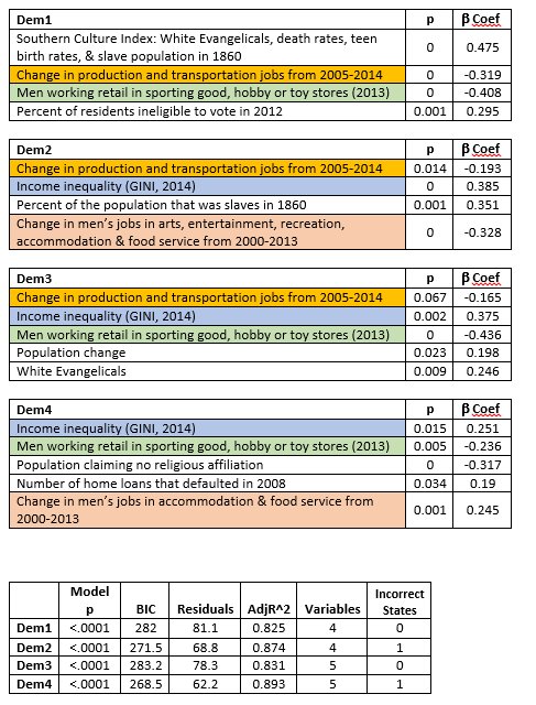
For my third round of creating primary prediction models for the presidential nomination, I focused just on the Democratic nomination between Clinton and Sanders. Here, I publish four new models, two of which correctly fit all 32 of the Democratic votes, and two that have only missed one vote.

I have not recalculated Republican-side models. Previously, I generated two models that had, as of March 23, correctly fit all states that had voted to that point. Aside from that, it looks like no matter what happens with the primary results, the GOP convention will become an open/brokered process. In that case, regression models about the primaries would be pointless, so I did not invest the time to recalculate them.

My last Democratic models, created just prior to the March 26 caucuses where Sanders swept Hawaii, Washington an Alaska in landslides, used 3 & 4 variables to correctly predict fit almost all of the states which had voted prior to those caucuses, and in all cases except one, correctly predicted these three wins for Sanders (one of the three models predicted a large Clinton win in Hawaii). The first of those three models, M1D, use unemployment (Dec 2015), no religious affiliation, out of state migration, and an average of the 2008-2012 presidential election votes, and so far has only 1 error, Iowa, out of the 32 states that have so far voted. The second model, MD2, so far has only 2 errors, Iowa & Oklahoma.

In these new models I do two things. First, I updated the algorithm to include the three states that have voted since I generated my last models. Second, I used the "numerically best" models, regardless of their application to theory. For the previous models I published, I ruled out those models that may have looked good on paper, but used obscure variables, like "number of men who worked in sports, hobby and toy stores in 2013," "women who work in the pharmaceutical retail stores," or "men who work in tobacco stores." While those are, to some degree, economic variables, and I was giving preference to economic variables, it is hard to make a broader theoretical cased based on these variables, since you would have to explain why these three specific job variables did a good job fitting the voting patterns, and the other 800 jobs variables had far less success. However, for these models, I throw theory to the wind, and include the obscure jobs variables. I filtered out those models that used more than two jobs variables.

There are some differences in predictions between these models, and the models from March 23. For example, in the previous models, Delaware was firmly in the Clinton camp, and both Rhode Island and West Virginia had two models putting them firmly in the Sanders camp. However, these new models put Delaware firmly for Sanders, and now the latter two are firmly showing for Clinton. There are several other states, like Maryland, New Jersey, New Mexico, South Dakota, and Wisconsin, where the previous models were contradictory, and solidly for either Sanders or Clinton now, or where they were previously showing a trend for one, but now are less clear. Given that the more recent models include more data, I would tend to support the findings of the newer models. However, MD1 from the first set of models still only has one incorrect state, and MD2 still only has two incorrect states.

One of the most common variables that appeared in the best models, is the income inequality variable, GINI, for 2014. As this value increases (approaches 1), it signifies more inequality, and as it decreases (approaches 0), it signifies more equality. In all of these models, the Beta coefficient is positive, meaning that as the value of this variable increases, the value of the dependent variable also increases. The dependent variable in this case is the difference between the Clinton and Sanders vote, as a subtraction (Clinton-Sanders), so is positive when Clinton wins, and negative when Sanders wins. What that implies is that in the states where you have greater levels of inequality, they are voting in larger numbers for Clinton. One might propose that poverty or education might be at work, rather than inequality, as such. However, several measures for poverty and education were included in the algorithm, and even accounting for those, income inequality is by far the more powerful predictor.

In a prior effort to find patterns in the data, I attempted to control for "cultural" factors, specifically, "Southern Culture," since there seemed to be early differences between Sanders vs Clinton wins based on the latter's southern victories. This Southern Culture Index did not make any of the previous best models. However, it was useful in one of the current models, Dem 1. As was previously shown, this index consists of four variables: % of White Evangelicals, death rates, teen birth rates, and slave population in 1860. A higher value means that state has stronger characteristics of "southern culture." Since the Southern Culture Index is positive in the Dem 1 model, it describes that the "more southern culture" a state has, the more likely it is to vote for Clinton. This result is fairly obvious just looking at a map of the Democratic contest so far. However, in the Dem1 model, what the results show is that it is the strongest of the four predictors.

In Dem2, the slave population variable is present by itself, and unsurprisingly given the results of the Southern Culture Index, as the slave population of 1860 increases, those states vote more strongly for Clinton. Similarly, in Dem 3, White Evangelicals appears as its own predictor, and like these other two, as they increase, so does support for Clinton. Conversely, hose that claim no religious affiliation appears in Dem4, and as expected, it is negative, showing that as this population is larger, that state votes more strongly for Sanders.

There are three jobs variables that made it into the final models: 1) "Change in production and transportation jobs from 2005-2014," 2) "Change in men's jobs in arts, entertainment, recreation, accommodation, & food service from 2000-2013,", and 3) men working retail in sporting goods, hobby, or toy stores in 2013." The most conservative way to interpret these results, when put into the context of the large number of jobs variables that were used to test models, is that the patterns in these jobs were just coincidentally, mathematically similar to the pattern of voting in the first 32 states which have voted so far this year. That may be the most one can say. Even if one were to assume that these results aren't simply a coincidence, one would still have to come up with a rationale for why, for example, when it comes to arts & food service jobs, the important factor was the change from 2000-2013, as opposed to 2005-2014. Similarly, one would have to explain why the production & transportation jobs change was important from 2005-2014, but not from 2000-2013. And why, of all of the possible job types, why these--why arts & food service, or why transportation & production? Perhaps there is a good explanation for these patterns, but I do not have one. My best guess is that it is coincidence, until other evidence is produced--for example, a good theory is presented, or the models correctly predict the rest of the state-level votes.

The jobs variables are mostly negative, meaning that as this value goes down, the dependent variable goes up, and vice versa. As jobs are lost over time, these variables become more negative, or as jobs increase over time, these variables become more positive. Since these values are mostly negative, presuming the results aren't simply a coincidence, it shows that in these states, as jobs in these specific fields are lost, they vote more strongly for Clinton. As jobs in these specific fields are gained, they vote more strongly for Sanders. One exception, is between Dem2 and Dem4. In Dem2, this is the broadest jobs variable in this sector--it includes arts, entertainment, recreation, accommodation, and food, and as these jobs are lost, that state votes more strongly for Clinton. However, in Dem4, this is just food and accommodation jobs. This variable is positive, meaning that as these jobs are lost, these states tend to vote more strongly for Sanders.

As before, I gave preference to those models that had the smallest residuals, the largest adjusted R-square, the lowest model p-values and variable p-values, the lowest BIC, and correctly fit the most states. All four models presented here have an adjusted R-square above 82%, and correctly predict either 31 or all 32 of the states that have voted as of April 2. All have model p-values less than 0.0001, and all variables have variance inflation factors less than 2.5. All individual variables have p<0.05, except for Dem 3, where one variable has p<0.07.