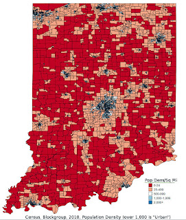
The first two images represent a "block-group" population density mapping of Indiana. The first of these images is an actual population density, derived directly from Census. While there is no variable for "population density," it can be readily calculated using "total population" divided by "land area." Population comes from the factfinder2 Census site linked above, and land area is embedded in the Tiger shapefile. There are various levels of measurement available from the Census, ranging from the entire US-level, all the way down to the block-level. In this case I have used the 2nd smallest unit available, the "block group" level, which is one step smaller than the "census tract" level. The calculated value can be transferred to the original Tiger block-group level shapefile and mapped through QGis. The Census definition of an urban space is one with 1,000 or more people per square mile. The Tiger shapefile gives the land area in square meters, so in order to get a square miles value, you must include a conversion factor. There are two primary sources in the Census for population--the annual ACS sample, and the decennial Census. The latter includes the entire population, while the former contains just a few individuals from each locality. The decennial Census allows more accurate reporting, and far smaller localities to be used. For this data I used the decennial Census.
The second image in this set is urban density, also derived solely from Census data. One of the values you can choose from the factfinder2 site, in addition to "population," is "urban" vs "rural." Within this set of information you can find 3 distinct values, in addition to the total population of the area. The first is "urbanized area" population, which is the number of people who live in regions with 50,000 or more people. The second is "urban cluster" population, with between 2,500-50,000 people. The third is "rural" population, with less than 2,500 people. The Census pre-defines these values based on the localization of the population density. This particular map is by block-group, and indicates the percent of people in each block group that occupy an "urbanized area." This is different from population density, in that the latter represents the total population/land area. Urban percent represents the percent of the population of an mapped feature (in this case a block-group) whose total incorporated area represents 50,000 or more people.
The final four images represent the Indiana state legislative districts, as highlighted by both population density and urban percent. The first two of these images is the lower house districts, while the last two are upper house districts. There are 100 lower house seats, and are analogous to the federal House of Representatives, while there are 50 upper house districts, analogous to the federal Senate. The Census Tiger shapefiles for these districts are drawn from the 2013 legislative maps. The population for the districts come directly from the Indiana web site, but the population density and urban percent had to be calculated by QGis, since the Census has not yet published either of these values for state legislative districts. I calculated these values by downloading the block-group-level population and urban data from factfinder2, and block-group-level shapefiles from Tiger, in addition to the state legislative shapefiles. In QGis there is a vector feature, "join attributes by location," which allows the user to spatially integrate various features. In this case, I used the spatial features of the state legislative districts, both upper and lower, respectively, as the digital shape targets, and "joined" to those shapes the population data in the block-group-level shapes from the second shapefile. Since there are many block-groups per legislative district, a join by "sum" allowed for a total population could be obtained for each of the districts.
The population density values were calculated directly from the land area given in the shapefiles for the legislative districts, and the population from the Indiana data for each legislative district. For this, QGis was not needed for calculations, just for mapping. In this case, as above, I used land area divided by total population, with the inclusion of the square meter to square miles conversion factor. However, for urban percent, I had to use the "join attributes by location" feature. After the join summed the values, the result was, for each legislative district, a sum of the population whom the census determined lived in an "urbanized area," as well as the total population for each district. The map colors thus represent the percent of people living in each district whom the Census has determined lives in an incorporated area of more than 50,000 people. This process sometimes has spatial difficulties--for example, block groups can cross legislative lines, and thus QGIS may produce unpredictable results in those instances. The summed populations did not match the populations given by the State of Indiana for each district. However, even if the population as such wasn't always accurate, the ratio of urban population to total population should be reasonably consistent with the spatial features. To test this, I compared the resulting urban percent values with the population density, which produced a correlation of r=0.78. I also did two separate comparisons, one using the census-tract level, and again with the block-group-level and the results were almost identical. For a finer comparison, a block-level measurement could be used, but that requires downloading separate files for each county, as opposed to one file for the entire state, and then integrating all of those county-level files back into one huge state file. For the purposes of this demonstration, the block-group-level files should be sufficient.


No comments:
Post a Comment